Circuits, gradients, and variational templates

Qiskit circuits, PennyLane gradients, mini VQC loop

The Problem

What practitioners underestimate

Even “fully quantum” variational algorithms spend most of wall-clock time in classical pre- and post-processing: transpilation, batching of shots, gradient accumulation, trust-region or Adam steps on parameters, logging, and checkpointing.

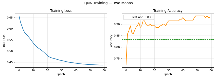
This chapter spends time on both Qiskit circuit composition and PennyLane’s differentiable execution before it frames chemistry or finance. The transferable skill is reading expectation traces and gradient norms as engineering signals.

You should leave this chapter able to

Construct a small parametrised circuit and verify it on a simulator.
Compute gradients of expectation values with respect to gate parameters.
Relate those gradients to an outer minimisation loop you could swap for business metrics later.

The Challenge

Depth, noise, and barren plateaus

The Challenge

Why shallow templates appear first

Deep unstructured ansätze are difficult to train under sampling noise. The workshop materials keep compact entangling layers so you can still interpret gradient magnitudes and loss curvature.

When you later connect to chemistry Hamiltonians, the same caution applies: more parameters do not automatically mean a better variational state. Subspace methods (SQD and relatives) exist precisely because full Hilbert-space paths are intractable.

Red flags during training

Flat gradients: update norms collapse while loss stalls—ansatz or encoding may be inadequate.

Inconsistent shots: changing shot counts mid-search invalidates comparisons.

Unverified transpilation: basis gates differ between simulator and claimed hardware target.

The Solution

One mini VQC training loop

The Solution

Pattern shared by VQE and QAOA

Choose parameters θ, prepare |ψ(θ)⟩, measure a cost operator (Hamiltonian for VQE, problem Hamiltonian for QAOA), feed the estimate to a classical optimiser, iterate. The companion code makes that loop tangible with a toy cost so the plumbing is visible.

Chemistry as motivation, not magic

Molecular Hamiltonians are genuine examples of the same pattern: Pauli sums that you measure term by term. Business QUBOs are different in origin but identical in the classical outer loop structure.

Training-style diagnostics reused as a metaphor for variational loss curves

Implementation

PennyLane expectation + classical step

Implementation

The excerpt mirrors the hybrid training pattern: a qnode returns an expectation, and PyTorch (or another AD framework) handles θ updates.

Swap PauliZ(0) for a Hamiltonian sum when you move to VQE; keep the outer loop identical.

Expectation-valued qnode (pattern)

import pennylane as qml
import torch
from torch import nn, optim

dev = qml.device("default.qubit", wires=n_qubits)

@qml.qnode(dev, interface="torch", diff_method="backprop")
def circuit(x, theta):
    qml.AngleEmbedding(x, wires=range(n_qubits))
    qml.StronglyEntanglingLayers(theta, wires=range(n_qubits))
    return qml.expval(qml.PauliZ(0))

theta = nn.Parameter(0.01 * torch.randn(depth, n_qubits, 3))
opt = optim.Adam([theta], lr=0.05)

for batch_x, batch_y in loader:
    preds = torch.stack([circuit(x, theta) for x in batch_x])
    loss = torch.nn.functional.mse_loss(preds, batch_y)
    opt.zero_grad()
    loss.backward()
    opt.step()

Companion code on GitHub

Summary

Carry the outer loop discipline forward

Summary

What to remember

Treat quantum modules as differentiable building blocks with the same logging standards as any neural submodule. If gradients vanish or shots explode, fix that before claiming domain advantage.

The next three chapters apply the same hybrid stack to a classifier, a finance portfolio, and a logistics route. The circuit skills here are the glue that keeps those later parts honest.

Continue this saga

Next chapter: Hybrid classifier stack.