The Challenge

Hypothesis class versus engineering cost

Replacing a classical MLP block with a quantum-inspired or quantum parameterised map can change which functions are easy to represent. It also changes optimisation noise, wall-clock time, and the burden on reviewers who must understand failure modes.

The defensible comparison holds the physics task fixed: same ODE, same boundary specification, same collocation schedule, same reported norm of the residual.

The Solution

Residual-first formulation

Let \(u_\theta(t)\) be the scalar network output. A damped harmonic template uses \(r(t)=\ddot u + \omega^2 u\). Collocation points sample \(t\) inside the domain; the PINN penalty is a mean squared residual plus boundary terms.

The companion workshop compares a purely classical PINN with a variant that routes part of the representational capacity through a small quantum circuit while keeping the same residual and boundary functional. Any claimed benefit must surface in that shared metric, not in auxiliary plots alone.

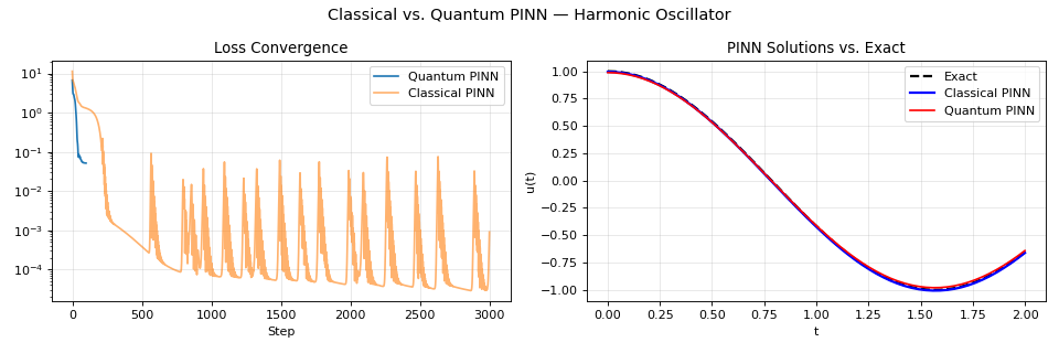
How to read the evidence plot

The companion figure compares training losses on the same task. Treat the vertical axis as a diagnostic: large drops early often reflect boundary correction, whereas the tail shows whether the residual continues to tighten or stalls because the ansatz cannot resolve high-frequency content.

Implementation

The discrete form below uses three time levels, explicit finite difference for \(\ddot u\), then a mean squared residual accumulated over the batch.

Swap in your boundary sampler and weight λ_bc; keep autograd enabled for θ.

import torch

def pinn_time_residual(model, t, dt, omega):
    u_prev = model(t - dt)
    u = model(t)
    u_next = model(t + dt)
    d2u = (u_next - 2.0 * u + u_prev) / (dt * dt)
    return d2u + (omega ** 2) * u

def pinn_loss(model, t_interior, dt, omega, t_bc, u_bc):
    r = pinn_time_residual(model, t_interior, dt, omega)
    loss_phys = torch.mean(r ** 2)
    u_hat = model(t_bc)
    loss_bc = torch.mean((u_hat - u_bc) ** 2)
    return loss_phys + lambda_bc * loss_bc

Log both loss_phys and loss_bc separately so reviewers can see which term dominates.

import torch

for t_colloc, t_bc, u_bc in batches:
    optim.zero_grad()
    loss = pinn_loss(model, t_colloc, dt, omega, t_bc, u_bc)
    loss.backward()
    optim.step()

Companion code on GitHub

Summary

Recorded run (illustrative)

In one logged training trace for the quantum-style variant, the total objective moved through roughly 6.73 → 1.96 → 0.14 → 0.065 → 0.053. Treat these as optimisation checkpoints, not magic constants: the useful statement is whether the residual keeps decreasing while boundary error stays bounded.

Takeaway for the rest of the saga

If a later chapter introduces a variational circuit, insist on the same discipline: name the quantity you minimise, show how it connects to the business or scientific constraint, and keep a classical reference implementation on the identical data and grid.